what is the minimum number of colors needed to color a tree? prove your claim.

Assignment of colors to elements of a graph subject to certain constraints.

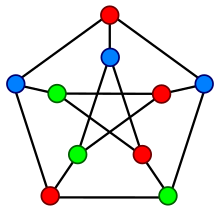
A proper vertex coloring of the Petersen graph with 3 colors, the minimum number possible.

In graph theory, graph coloring is a special example of graph labeling; information technology is an assignment of labels traditionally called "colors" to elements of a graph subject field to sure constraints. In its simplest form, information technology is a way of coloring the vertices of a graph such that no ii adjacent vertices are of the same color; this is called a vertex coloring. Similarly, an border coloring assigns a color to each edge so that no two adjacent edges are of the same color, and a face coloring of a planar graph assigns a colour to each face or region so that no two faces that share a purlieus have the same color.

Vertex coloring is often used to introduce graph coloring problems, since other coloring issues can exist transformed into a vertex coloring instance. For example, an edge coloring of a graph is simply a vertex coloring of its line graph, and a face coloring of a plane graph is merely a vertex coloring of its dual. Notwithstanding, non-vertex coloring problems are ofttimes stated and studied as-is. This is partly pedagogical, and partly considering some problems are best studied in their non-vertex form, as in the case of border coloring.

The convention of using colors originates from coloring the countries of a map, where each face up is literally colored. This was generalized to coloring the faces of a graph embedded in the plane. By planar duality information technology became coloring the vertices, and in this class it generalizes to all graphs. In mathematical and computer representations, it is typical to use the first few positive or non-negative integers equally the "colors". In general, 1 tin apply any finite gear up as the "color set". The nature of the coloring problem depends on the number of colors just not on what they are.

Graph coloring enjoys many practical applications as well as theoretical challenges. Abreast the classical types of problems, different limitations can too exist set on the graph, or on the style a color is assigned, or fifty-fifty on the colour itself. It has even reached popularity with the general public in the form of the popular number puzzle Sudoku. Graph coloring is still a very active field of enquiry.

Note: Many terms used in this article are defined in Glossary of graph theory.

History [edit]

The starting time results near graph coloring deal almost exclusively with planar graphs in the form of the coloring of maps. While trying to colour a map of the counties of England, Francis Guthrie postulated the four colour theorize, noting that iv colors were sufficient to color the map so that no regions sharing a common border received the aforementioned color. Guthrie'south brother passed on the question to his mathematics teacher Augustus de Morgan at University Higher, who mentioned it in a letter to William Hamilton in 1852. Arthur Cayley raised the problem at a meeting of the London Mathematical Social club in 1879. The same year, Alfred Kempe published a paper that claimed to found the result, and for a decade the 4 color problem was considered solved. For his accomplishment Kempe was elected a Fellow of the Majestic Society and later President of the London Mathematical Gild.^[1]

In 1890, Heawood pointed out that Kempe'southward argument was wrong. However, in that newspaper he proved the five color theorem, saying that every planar map can be colored with no more than than 5 colors, using ideas of Kempe. In the following century, a vast corporeality of piece of work and theories were developed to reduce the number of colors to four, until the 4 color theorem was finally proved in 1976 by Kenneth Appel and Wolfgang Haken. The proof went back to the ideas of Heawood and Kempe and largely disregarded the intervening developments.^[2] The proof of the four colour theorem is likewise noteworthy for being the first major reckoner-aided proof.

In 1912, George David Birkhoff introduced the chromatic polynomial to report the coloring problems, which was generalised to the Tutte polynomial by Tutte, important structures in algebraic graph theory. Kempe had already drawn attention to the general, not-planar example in 1879,^[3] and many results on generalisations of planar graph coloring to surfaces of college lodge followed in the early on 20th century.

In 1960, Claude Berge formulated another theorize about graph coloring, the strong perfect graph conjecture, originally motivated by an information-theoretic concept called the goose egg-error chapters of a graph introduced by Shannon. The conjecture remained unresolved for xl years, until it was established as the celebrated strong perfect graph theorem by Chudnovsky, Robertson, Seymour, and Thomas in 2002.

Graph coloring has been studied as an algorithmic trouble since the early 1970s: the chromatic number trouble (run across below) is ane of Karp's 21 NP-complete problems from 1972, and at approximately the same fourth dimension various exponential-time algorithms were developed based on backtracking and on the deletion-contraction recurrence of Zykov (1949). One of the major applications of graph coloring, annals allotment in compilers, was introduced in 1981.

Definition and terminology [edit]

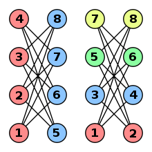
This graph can be iii-colored in 12 different means.

Vertex coloring [edit]

When used without any qualification, a coloring of a graph is about e'er a proper vertex coloring, namely a labeling of the graph'south vertices with colors such that no two vertices sharing the same border accept the same color. Since a vertex with a loop (i.east. a connection directly back to itself) could never exist properly colored, information technology is understood that graphs in this context are loopless.

The terminology of using colors for vertex labels goes dorsum to map coloring. Labels like cherry-red and blue are only used when the number of colors is small, and normally it is understood that the labels are drawn from the integers {1, two, 3, ...}.

A coloring using at most k colors is called a (proper) m-coloring. The smallest number of colors needed to colour a graph One thousand is called its chromatic number, and is often denoted χ(G). Sometimes γ(1000) is used, since χ(G) is also used to announce the Euler characteristic of a graph. A graph that can exist assigned a (proper) k-coloring is k-colorable, and information technology is k-chromatic if its chromatic number is exactly grand. A subset of vertices assigned to the same color is called a colour class, every such course forms an independent set. Thus, a k-coloring is the same as a partition of the vertex set into yard contained sets, and the terms k-partite and g-colorable have the same meaning.

Chromatic polynomial [edit]

All not-isomorphic graphs on 3 vertices and their chromatic polynomials. The empty graph Due east _three (red) admits a 1-coloring; the complete graph M _iii (blue) admits a 3-coloring; the other graphs admit a 2-coloring.

The chromatic polynomial counts the number of ways a graph can be colored using some of a given number of colors. For example, using three colors, the graph in the adjacent image tin be colored in 12 ways. With only ii colors, it cannot exist colored at all. With iv colors, it can exist colored in 24 + four⋅12 = 72 ways: using all four colors, there are four! = 24 valid colorings (every assignment of 4 colors to any 4-vertex graph is a proper coloring); and for every pick of 3 of the 4 colors, there are 12 valid 3-colorings. And so, for the graph in the example, a table of the number of valid colorings would start like this:

Bachelor colors	ane	2	3	4	…
Number of colorings	0	0	12	72	…

The chromatic polynomial is a function ${\displaystyle P(G,t)}$ that counts the number of t-colorings of Grand. As the name indicates, for a given G the function is indeed a polynomial in t. For the example graph, ${\displaystyle P(Grand,t)=t(t-i)^{2}(t-two)}$ , and indeed ${\displaystyle P(Chiliad,four)=72}$ .

The chromatic polynomial includes more than information about the colorability of G than does the chromatic number. Indeed, χ is the smallest positive integer that is not a nothing of the chromatic polynomial:

${\displaystyle \chi (G)=\min\{thou\,\colon \,P(G,k)>0\}.}$

Chromatic polynomials for certain graphs

Triangle K 3	${\displaystyle t(t-one)(t-2)}$
Complete graph K n	${\displaystyle t(t-1)(t-2)\cdots (t-(n-1))}$
Tree with n vertices	${\displaystyle t(t-i)^{n-one}}$
Bike C n	${\displaystyle (t-1)^{n}+(-1)^{n}(t-1)}$
Petersen graph	${\displaystyle t(t-i)(t-two)(t^{7}-12t^{half-dozen}+67t^{5}-230t^{4}+529t^{3}-814t^{2}+775t-352)}$

Edge coloring [edit]

An edge coloring of a graph is a proper coloring of the edges, meaning an consignment of colors to edges so that no vertex is incident to two edges of the aforementioned color. An edge coloring with thou colors is called a k-border-coloring and is equivalent to the trouble of segmentation the edge set into k matchings. The smallest number of colors needed for an edge coloring of a graph G is the chromatic alphabetize, or edge chromatic number, χ′(G). A Tait coloring is a iii-edge coloring of a cubic graph. The iv color theorem is equivalent to the exclamation that every planar cubic bridgeless graph admits a Tait coloring.

Total coloring [edit]

Total coloring is a type of coloring on the vertices and edges of a graph. When used without any qualification, a full coloring is always assumed to be proper in the sense that no next vertices, no side by side edges, and no edge and its stop-vertices are assigned the aforementioned color. The total chromatic number χ″(G) of a graph G is the fewest colors needed in any full coloring of Grand.

Unlabeled coloring [edit]

An unlabeled coloring of a graph is an orbit of a coloring under the action of the automorphism group of the graph. Note that the colors remain labeled; it is the graph that is unlabeled. In that location is an counterpart of the chromatic polynomial which counts the number of unlabeled colorings of a graph from a given finite color gear up.

If we interpret a coloring of a graph on ${\displaystyle d}$ vertices as a vector in ${\displaystyle \mathbb {Z} ^{d}}$ , the activity of an automorphism is a permutation of the coefficients in the coloring vector.

Properties [edit]

Upper bounds on the chromatic number [edit]

Assigning distinct colors to distinct vertices ever yields a proper coloring, so

${\displaystyle 1\leq \chi (G)\leq n.}$

The but graphs that can exist 1-colored are edgeless graphs. A complete graph ${\displaystyle K_{n}}$ of n vertices requires ${\displaystyle \chi (K_{n})=n}$ colors. In an optimal coloring at that place must be at to the lowest degree one of the graph's m edges between every pair of color classes, and then

${\displaystyle \chi (G)(\chi (G)-1)\leq 2m.}$

If G contains a clique of size k, then at to the lowest degree k colors are needed to color that clique; in other words, the chromatic number is at to the lowest degree the clique number:

${\displaystyle \chi (G)\geq \omega (G).}$

For perfect graphs this bound is tight. Finding cliques is known every bit the clique problem.

More more often than not a family ${\displaystyle {\mathcal {F}}}$ of graphs is ${\displaystyle \chi }$ -bounded if there is some function ${\displaystyle c}$ such that the graphs ${\displaystyle G}$ in ${\displaystyle {\mathcal {F}}}$ tin be colored with at most ${\displaystyle c(\omega (G))}$ colors, for the family of the perfect graphs this function is ${\displaystyle c(\omega (Thousand))=\omega (Chiliad)}$ .

The ii-colorable graphs are exactly the bipartite graphs, including trees and forests. By the four color theorem, every planar graph tin can exist 4-colored.

A greedy coloring shows that every graph can be colored with one more color than the maximum vertex degree,

${\displaystyle \chi (G)\leq \Delta (Chiliad)+1.}$

Complete graphs take ${\displaystyle \chi (Thou)=n}$ and ${\displaystyle \Delta (M)=n-one}$ , and odd cycles have ${\displaystyle \chi (Thousand)=three}$ and ${\displaystyle \Delta (Grand)=2}$ , so for these graphs this jump is best possible. In all other cases, the bound can be slightly improved; Brooks' theorem^[4] states that

Brooks' theorem: ${\displaystyle \chi (One thousand)\leq \Delta (G)}$ for a continued, simple graph G, unless G is a complete graph or an odd cycle.

Lower bounds on the chromatic number [edit]

Several lower bounds for the chromatic premises have been discovered over the years:

Hoffman's leap: Let ${\displaystyle W}$ exist a existent symmetric matrix such that ${\displaystyle W_{i,j}=0}$ whenever ${\displaystyle (i,j)}$ is not an edge in ${\displaystyle G}$ . Define ${\displaystyle \chi _{Due west}(1000)=1-{\tfrac {\lambda _{\max }(W)}{\lambda _{\min }(W)}}}$ , where ${\displaystyle \lambda _{\max }(W),\lambda _{\min }(Westward)}$ are the largest and smallest eigenvalues of ${\displaystyle Westward}$ . Ascertain ${\textstyle \chi _{H}(Yard)=\max _{West}\chi _{Due west}(Grand)}$ , with ${\displaystyle W}$ as above. And then:

${\displaystyle \chi _{H}(G)\leq \chi (K).}$

Vector chromatic number : Let ${\displaystyle W}$ be a positive semi-definite matrix such that ${\displaystyle W_{i,j}\leq -{\tfrac {1}{thou-one}}}$ whenever ${\displaystyle (i,j)}$ is an border in ${\displaystyle G}$ . Define ${\displaystyle \chi _{V}(G)}$ to be the least k for which such a matrix ${\displaystyle W}$ exists. So

${\displaystyle \chi _{V}(Thousand)\leq \chi (G).}$

Lovász number: The Lovász number of a complementary graph is also a lower leap on the chromatic number:

${\displaystyle \vartheta ({\bar {Thou}})\leq \chi (Grand).}$

Partial chromatic number: The fractional chromatic number of a graph is a lower bound on the chromatic number besides:

${\displaystyle \chi _{f}(G)\leq \chi (G).}$

These bounds are ordered as follows:

${\displaystyle \chi _{H}(G)\leq \chi _{V}(M)\leq \vartheta ({\bar {G}})\leq \chi _{f}(M)\leq \chi (G).}$

Graphs with high chromatic number [edit]

Graphs with large cliques take a high chromatic number, but the opposite is not true. The Grötzsch graph is an example of a 4-chromatic graph without a triangle, and the example tin be generalized to the Mycielskians.

Theorem (William T. Tutte 1947,^[five] Alexander Zykov 1949, January Mycielski 1955): There exist triangle-gratuitous graphs with arbitrarily high chromatic number.

To prove this, both, Mycielski and Zykov, each gave a structure of an inductively defined family of triangle-free graphs but with arbitrarily large chromatic number.^[six] Burling (1965)^[7] constructed axis aligned boxes in ${\displaystyle \mathbb {R} ^{3}}$ whose intersection graph is triangle-gratuitous and requires arbitrarily many colors to be properly colored. This family of graphs is and then chosen the Burling graphs. The same class of graphs is used for the construction of a family unit of triangle-free line segments in the plane, given past Pawlik et. al. (2014).^[8] It shows that the chromatic number of its intersection graph is arbitrarily large as well. Hence, this implies that axis aligned boxes in ${\displaystyle \mathbb {R} ^{3}}$ every bit well every bit line segments in ${\displaystyle \mathbb {R} ^{2}}$ are non χ-divisional.^[eight]

From Brooks's theorem, graphs with high chromatic number must have high maximum degree. But colorability is not an entirely local miracle: A graph with high girth looks locally like a tree, because all cycles are long, but its chromatic number need not be 2:

Theorem (Erdős): There be graphs of arbitrarily high girth and chromatic number.^[9]

Bounds on the chromatic index [edit]

An edge coloring of G is a vertex coloring of its line graph ${\displaystyle L(G)}$ , and vice versa. Thus,

${\displaystyle \chi '(G)=\chi (Fifty(G)).}$

There is a potent relationship between edge colorability and the graph's maximum degree ${\displaystyle \Delta (Yard)}$ . Since all edges incident to the aforementioned vertex need their own color, we have

${\displaystyle \chi '(1000)\geq \Delta (G).}$

Moreover,

Kőnig'southward theorem: ${\displaystyle \chi '(Yard)=\Delta (G)}$ if Thou is bipartite.

In general, the human relationship is fifty-fifty stronger than what Brooks'south theorem gives for vertex coloring:

Vizing's Theorem: A graph of maximal degree ${\displaystyle \Delta }$ has edge-chromatic number ${\displaystyle \Delta }$ or ${\displaystyle \Delta +1}$ .

Other properties [edit]

A graph has a k-coloring if and simply if it has an acyclic orientation for which the longest path has length at nigh k; this is the Gallai–Hasse–Roy–Vitaver theorem (Nešetřil & Ossona de Mendez 2012).

For planar graphs, vertex colorings are substantially dual to nowhere-nothing flows.

About infinite graphs, much less is known. The following are two of the few results about infinite graph coloring:

• If all finite subgraphs of an space graph G are g-colorable, and then and then is One thousand, under the assumption of the axiom of option. This is the de Bruijn–Erdős theorem of de Bruijn & Erdős (1951).
• If a graph admits a total n-coloring for every north ≥ northward ₀, it admits an infinite full coloring (Fawcett 1978).

Open bug [edit]

As stated to a higher place, ${\displaystyle \omega (G)\leq \chi (G)\leq \Delta (Chiliad)+1.}$ A conjecture of Reed from 1998 is that the value is essentially closer to the lower bound, ${\displaystyle \chi (Chiliad)\leq \left\lceil {\frac {\omega (G)+\Delta (G)+ane}{2}}\right\rceil .}$

The chromatic number of the plane, where two points are side by side if they take unit distance, is unknown, although it is one of 5, half-dozen, or 7. Other open problems concerning the chromatic number of graphs include the Hadwiger conjecture stating that every graph with chromatic number k has a complete graph on k vertices every bit a pocket-size, the Erdős–Faber–Lovász conjecture bounding the chromatic number of unions of complete graphs that accept at nigh 1 vertex in common to each pair, and the Albertson theorize that among thou-chromatic graphs the complete graphs are the ones with smallest crossing number.

When Birkhoff and Lewis introduced the chromatic polynomial in their attack on the four-colour theorem, they conjectured that for planar graphs M, the polynomial ${\displaystyle P(K,t)}$ has no zeros in the region ${\displaystyle [4,\infty )}$ . Although it is known that such a chromatic polynomial has no zeros in the region ${\displaystyle [5,\infty )}$ and that ${\displaystyle P(Grand,4)\neq 0}$ , their conjecture is notwithstanding unresolved. It also remains an unsolved problem to characterize graphs which have the aforementioned chromatic polynomial and to determine which polynomials are chromatic.

Algorithms [edit]

Graph coloring
Determination
Name	Graph coloring, vertex coloring, k-coloring
Input	Graph M with north vertices. Integer g
Output	Does G acknowledge a proper vertex coloring with k colors?
Running time	O(2due north northward)[10]
Complexity	NP-complete
Reduction from	3-Satisfiability
Garey–Johnson	GT4
Optimisation
Proper noun	Chromatic number
Input	Graph Chiliad with n vertices.
Output	χ(G)
Complication	NP-hard
Approximability	O(n (log due north)−3(log log northward)ii)
Inapproximability	O(n 1−ε) unless P = NP
Counting problem
Proper noun	Chromatic polynomial
Input	Graph G with northward vertices. Integer k
Output	The number P (G,g) of proper m-colorings of K
Running time	O(2n n)
Complication	#P-complete
Approximability	FPRAS for restricted cases
Inapproximability	No PTAS unless P = NP

Polynomial time [edit]

Determining if a graph can exist colored with 2 colors is equivalent to determining whether or non the graph is bipartite, and thus computable in linear time using breadth-kickoff search or depth-beginning search. More generally, the chromatic number and a corresponding coloring of perfect graphs can be computed in polynomial time using semidefinite programming. Closed formulas for chromatic polynomial are known for many classes of graphs, such equally forests, chordal graphs, cycles, wheels, and ladders, so these tin can be evaluated in polynomial time.

If the graph is planar and has depression branch-width (or is nonplanar only with a known branch decomposition), then it can be solved in polynomial time using dynamic programming. In full general, the time required is polynomial in the graph size, but exponential in the branch-width.

Exact algorithms [edit]

Animal-force search for a k-coloring considers each of the ${\displaystyle k^{northward}}$ assignments of grand colors to n vertices and checks for each if it is legal. To compute the chromatic number and the chromatic polynomial, this process is used for every ${\displaystyle one thousand=1,\ldots ,due north-1}$ , impractical for all merely the smallest input graphs.

Using dynamic programming and a bound on the number of maximal independent sets, k-colorability can be decided in time and space ${\displaystyle O(2.4423^{n})}$ .^[xi] Using the principle of inclusion–exclusion and Yates's algorithm for the fast zeta transform, g-colorability can be decided in fourth dimension ${\displaystyle O(2^{due north}northward)}$ ^[10] for any grand. Faster algorithms are known for 3- and four-colorability, which can be decided in time ${\displaystyle O(1.3289^{n})}$ ^[12] and ${\displaystyle O(1.7272^{n})}$ ,^[13] respectively. Exponentially faster algorithms are besides known for 5- and half dozen-colorability, also as for restricted families of graphs, including sparse graphs.^[14]

Wrinkle [edit]

The contraction ${\displaystyle Grand/uv}$ of a graph Grand is the graph obtained past identifying the vertices u and v, and removing any edges betwixt them. The remaining edges originally incident to u or five are now incident to their identification. This functioning plays a major office in the assay of graph coloring.

The chromatic number satisfies the recurrence relation:

${\displaystyle \chi (G)={\text{min}}\{\chi (Yard+uv),\chi (G/uv)\}}$

due to Zykov (1949), where u and v are not-adjacent vertices, and ${\displaystyle G+uv}$ is the graph with the edge uv added. Several algorithms are based on evaluating this recurrence and the resulting ciphering tree is sometimes called a Zykov tree. The running time is based on a heuristic for choosing the vertices u and v.

The chromatic polynomial satisfies the post-obit recurrence relation

${\displaystyle P(1000-uv,k)=P(Thou/uv,yard)+P(G,chiliad)}$

where u and v are adjacent vertices, and ${\displaystyle 1000-uv}$ is the graph with the edge uv removed. ${\displaystyle P(G-uv,grand)}$ represents the number of possible proper colorings of the graph, where the vertices may take the same or different colors. Then the proper colorings arise from two different graphs. To explain, if the vertices u and v take different colors, and so we might every bit well consider a graph where u and v are next. If u and 5 take the aforementioned colors, we might too consider a graph where u and v are contracted. Tutte's marvel about which other graph backdrop satisfied this recurrence led him to discover a bivariate generalization of the chromatic polynomial, the Tutte polynomial.

These expressions give rise to a recursive process called the deletion–contraction algorithm, which forms the basis of many algorithms for graph coloring. The running time satisfies the aforementioned recurrence relation as the Fibonacci numbers, so in the worst case the algorithm runs in time inside a polynomial gene of ${\displaystyle \left({\tfrac {i+{\sqrt {5}}}{ii}}\right)^{northward+yard}=O(1.6180^{n+m})}$ for n vertices and grand edges.^[xv] The analysis tin can be improved to inside a polynomial factor of the number ${\displaystyle t(G)}$ of spanning copse of the input graph.^[16] In do, co-operative and jump strategies and graph isomorphism rejection are employed to avoid some recursive calls. The running fourth dimension depends on the heuristic used to pick the vertex pair.

Greedy coloring [edit]

Two greedy colorings of the same graph using different vertex orders. The correct example generalizes to ii-colorable graphs with n vertices, where the greedy algorithm expends ${\displaystyle n/2}$ colors.

The greedy algorithm considers the vertices in a specific order ${\displaystyle v_{1}}$ ,…, ${\displaystyle v_{northward}}$ and assigns to ${\displaystyle v_{i}}$ the smallest bachelor color non used by ${\displaystyle v_{i}}$ 's neighbours amid ${\displaystyle v_{ane}}$ ,…, ${\displaystyle v_{i-1}}$ , calculation a fresh color if needed. The quality of the resulting coloring depends on the chosen ordering. There exists an ordering that leads to a greedy coloring with the optimal number of ${\displaystyle \chi (K)}$ colors. On the other hand, greedy colorings tin be arbitrarily bad; for example, the crown graph on north vertices tin be ii-colored, but has an ordering that leads to a greedy coloring with ${\displaystyle n/ii}$ colors.

For chordal graphs, and for special cases of chordal graphs such as interval graphs and indifference graphs, the greedy coloring algorithm can exist used to observe optimal colorings in polynomial time, by choosing the vertex ordering to exist the reverse of a perfect elimination ordering for the graph. The perfectly orderable graphs generalize this property, but it is NP-hard to find a perfect ordering of these graphs.

If the vertices are ordered co-ordinate to their degrees, the resulting greedy coloring uses at near ${\displaystyle {\text{max}}_{i}{\text{ min}}\{d(x_{i})+1,i\}}$ colors, at most one more than the graph'southward maximum degree. This heuristic is sometimes called the Welsh–Powell algorithm.^[17] Another heuristic due to Brélaz establishes the ordering dynamically while the algorithm proceeds, choosing next the vertex adjacent to the largest number of unlike colors.^[18] Many other graph coloring heuristics are similarly based on greedy coloring for a specific static or dynamic strategy of ordering the vertices, these algorithms are sometimes called sequential coloring algorithms.

The maximum (worst) number of colors that tin be obtained by the greedy algorithm, by using a vertex ordering chosen to maximize this number, is called the Grundy number of a graph.

Heuristic algorithms [edit]

Two well-known polynomial-fourth dimension heuristics for graph colouring are the DSatur and recursive largest offset (RLF) algorithms.

Similarly to the greedy colouring algorithm, DSatur colours the vertices of a graph 1 after another, expending a previously unused colour when needed. Once a new vertex has been coloured, the algorithm determines which of the remaining uncoloured vertices has the highest number of different colours in its neighbourhood and colours this vertex side by side. This is defined every bit the degree of saturation of a given vertex.

The recursive largest first algorithm operates in a unlike style past constructing each color course i at a time. It does this by identifying a maximal independent set of vertices in the graph using specialised heuristic rules. It then assigns these vertices to the same color and removes them from the graph. These actions are repeated on the remaining subgraph until no vertices remain.

The worst-example complication of DSatur is ${\displaystyle O(n^{2})}$ , where ${\displaystyle north}$ is the number of vertices in the graph. The algorithm can also exist implemented using a binary heap to store saturation degrees, operating in ${\displaystyle O((due north+m)\log northward)}$ where ${\displaystyle yard}$ is the number of edges in the graph.^[nineteen] This produces much faster runs with sparse graphs. The overall complication of RLF is slightly higher than DSatur at ${\displaystyle {\mathcal {O}}(mn)}$ .^[nineteen]

DSatur and RLF are exact for bipartite, cycle, and wheel graphs.^[xix]

Parallel and distributed algorithms [edit]

In the field of distributed algorithms, graph coloring is closely related to the problem of symmetry breaking. The electric current state-of-the-art randomized algorithms are faster for sufficiently big maximum degree Δ than deterministic algorithms. The fastest randomized algorithms employ the multi-trials technique by Schneider et al.^[xx]

In a symmetric graph, a deterministic distributed algorithm cannot notice a proper vertex coloring. Some auxiliary information is needed in gild to intermission symmetry. A standard assumption is that initially each node has a unique identifier, for example, from the fix {1, 2, ..., n}. Put otherwise, we assume that nosotros are given an northward-coloring. The challenge is to reduce the number of colors from n to, due east.m., Δ + i. The more colors are employed, eastward.1000. O(Δ) instead of Δ + 1, the fewer advice rounds are required.^[20]

A straightforward distributed version of the greedy algorithm for (Δ + i)-coloring requires Θ(n) advice rounds in the worst case − information may need to be propagated from 1 side of the network to some other side.

The simplest interesting case is an north-bicycle. Richard Cole and Uzi Vishkin^[21] show that at that place is a distributed algorithm that reduces the number of colors from n to O(logn) in i synchronous communication step. By iterating the same procedure, it is possible to obtain a iii-coloring of an n-cycle in O(log*n) communication steps (assuming that we have unique node identifiers).

The function log*, iterated logarithm, is an extremely slowly growing role, "well-nigh constant". Hence the result past Cole and Vishkin raised the question of whether there is a constant-time distributed algorithm for 3-coloring an due north-cycle. Linial (1992) showed that this is not possible: any deterministic distributed algorithm requires Ω(log*north) communication steps to reduce an n-coloring to a 3-coloring in an n-cycle.

The technique by Cole and Vishkin tin be applied in arbitrary bounded-caste graphs besides; the running fourth dimension is poly(Δ) + O(log*north).^[22] The technique was extended to unit disk graphs by Schneider et al.^[23] The fastest deterministic algorithms for (Δ + i)-coloring for minor Δ are due to Leonid Barenboim, Michael Elkin and Fabian Kuhn.^[24] The algorithm by Barenboim et al. runs in fourth dimension O(Δ) + log*(n)/2, which is optimal in terms of n since the constant factor 1/2 cannot be improved due to Linial's lower bound. Panconesi & Srinivasan (1996) apply network decompositions to compute a Δ+1 coloring in time ${\displaystyle 2^{O\left({\sqrt {\log n}}\correct)}}$ .

The problem of edge coloring has also been studied in the distributed model. Panconesi & Rizzi (2001) achieve a (2Δ − one)-coloring in O(Δ + log*n) time in this model. The lower leap for distributed vertex coloring due to Linial (1992) applies to the distributed edge coloring problem as well.

Decentralized algorithms [edit]

Decentralized algorithms are ones where no message passing is allowed (in contrast to distributed algorithms where local message passing takes places), and efficient decentralized algorithms exist that will colour a graph if a proper coloring exists. These assume that a vertex is able to sense whether whatsoever of its neighbors are using the same color every bit the vertex i.east., whether a local conflict exists. This is a balmy assumption in many applications e.thousand. in wireless channel resource allotment information technology is usually reasonable to assume that a station will be able to detect whether other interfering transmitters are using the same aqueduct (e.g. by measuring the SINR). This sensing information is sufficient to permit algorithms based on learning automata to find a proper graph coloring with probability 1.^[25]

Computational complication [edit]

Graph coloring is computationally hard. It is NP-consummate to decide if a given graph admits a k-coloring for a given k except for the cases thou ∈ {0,1,2} . In particular, it is NP-hard to compute the chromatic number.^[26] The 3-coloring problem remains NP-consummate even on 4-regular planar graphs.^[27] Still, for every k > iii, a k-coloring of a planar graph exists by the iv color theorem, and information technology is possible to observe such a coloring in polynomial fourth dimension.

The best known approximation algorithm computes a coloring of size at most inside a factor O(n(log logn)ⁱⁱ(log n)^−three) of the chromatic number.^[28] For all ε > 0, approximating the chromatic number within n ^one−ε is NP-hard.^[29]

It is also NP-hard to color a iii-colorable graph with iv colors^[30] and a thousand-colorable graph with k ^{(log k ) / 25} colors for sufficiently large constant grand.^[31]

Computing the coefficients of the chromatic polynomial is #P-hard. In fact, fifty-fifty computing the value of ${\displaystyle \chi (G,k)}$ is #P-hard at any rational point k except for k = 1 and grand = 2.^[32] At that place is no FPRAS for evaluating the chromatic polynomial at any rational point k ≥ 1.5 except for grand = 2 unless NP = RP.^[33]

For border coloring, the proof of Vizing's upshot gives an algorithm that uses at almost Δ+ane colors. Still, deciding between the ii candidate values for the edge chromatic number is NP-consummate.^[34] In terms of approximation algorithms, Vizing'due south algorithm shows that the edge chromatic number tin can exist approximated to inside 4/3, and the hardness upshot shows that no (4/iii −ε )-algorithm exists for any ε > 0 unless P = NP. These are among the oldest results in the literature of approximation algorithms, even though neither newspaper makes explicit use of that notion.^[35]

Applications [edit]

Scheduling [edit]

Vertex coloring models to a number of scheduling problems.^[36] In the cleanest grade, a given set up of jobs need to be assigned to time slots, each job requires ane such slot. Jobs can be scheduled in any guild, but pairs of jobs may be in conflict in the sense that they may not be assigned to the aforementioned time slot, for example because they both rely on a shared resource. The corresponding graph contains a vertex for every job and an border for every conflicting pair of jobs. The chromatic number of the graph is exactly the minimum makespan, the optimal time to end all jobs without conflicts.

Details of the scheduling problem define the structure of the graph. For example, when assigning shipping to flights, the resulting conflict graph is an interval graph, then the coloring trouble can be solved efficiently. In bandwidth allocation to radio stations, the resulting disharmonize graph is a unit disk graph, so the coloring problem is three-approximable.

Register allocation [edit]

A compiler is a estimator program that translates one reckoner language into some other. To ameliorate the execution time of the resulting lawmaking, one of the techniques of compiler optimization is register allocation, where the most frequently used values of the compiled program are kept in the fast processor registers. Ideally, values are assigned to registers so that they can all reside in the registers when they are used.

The textbook approach to this trouble is to model it as a graph coloring trouble.^[37] The compiler constructs an interference graph, where vertices are variables and an edge connects two vertices if they are needed at the aforementioned fourth dimension. If the graph tin can be colored with k colors then whatever set of variables needed at the same fourth dimension can exist stored in at most k registers.

Other applications [edit]

The problem of coloring a graph arises in many practical areas such as pattern matching, sports scheduling, designing seating plans, exam timetabling, the scheduling of taxis, and solving Sudoku puzzles.^[19]

Other colorings [edit]

Ramsey theory [edit]

An important course of improper coloring bug is studied in Ramsey theory, where the graph'due south edges are assigned to colors, and in that location is no restriction on the colors of incident edges. A simple example is the friendship theorem, which states that in whatsoever coloring of the edges of ${\displaystyle K_{6}}$ , the complete graph of half dozen vertices, there volition be a monochromatic triangle; often illustrated by saying that any group of six people either has 3 mutual strangers or three mutual acquaintances. Ramsey theory is concerned with generalisations of this idea to seek regularity amid disorder, finding full general conditions for the existence of monochromatic subgraphs with given structure.

Other colorings [edit]

Adjacent-vertex-distinguishing-total coloring A full coloring with the additional restriction that any two side by side vertices have different color sets Acyclic coloring Every 2-chromatic subgraph is acyclic B-coloring a coloring of the vertices where each color class contains a vertex that has a neighbour in all other colour classes. Circular coloring Motivated by task systems in which production proceeds in a cyclic fashion Cocoloring An improper vertex coloring where every color class induces an independent set or a clique Complete coloring Every pair of colors appears on at least one edge Defective coloring An improper vertex coloring where every color course induces a bounded caste subgraph. Distinguishing coloring An improper vertex coloring that destroys all the symmetries of the graph Equitable coloring The sizes of colour classes differ past at near i Exact coloring Every pair of colors appears on exactly one border Partial coloring Vertices may have multiple colors, and on each edge the sum of the color parts of each vertex is not greater than one Hamiltonian coloring Uses the length of the longest path between ii vertices, also known as the detour distance Harmonious coloring Every pair of colors appears on at near 1 edge Incidence coloring Each adjacent incidence of vertex and border is colored with distinct colors Interval edge coloring A color of edges coming together in a common vertex must be face-to-face List coloring Each vertex chooses from a listing of colors Listing border-coloring Each edge chooses from a listing of colors L(h, thou)-coloring Difference of colors at adjacent vertices is at least h and deviation of colors of vertices at a distance two is at least thousand. A particular example is Fifty(two,1)-coloring.

Oriented coloring Takes into account orientation of edges of the graph Path coloring Models a routing trouble in graphs Radio coloring Sum of the distance between the vertices and the difference of their colors is greater than one thousand+1, where k is a positive integer. Rank coloring If 2 vertices take the same color i, then every path betwixt them contain a vertex with colour greater than i Subcoloring An improper vertex coloring where every color form induces a union of cliques Sum coloring The benchmark of minimalization is the sum of colors Star coloring Every 2-chromatic subgraph is a disjoint collection of stars Strong coloring Every color appears in every partition of equal size exactly in one case Potent edge coloring Edges are colored such that each color course induces a matching (equivalent to coloring the square of the line graph) T-coloring Absolute value of the difference betwixt two colors of adjacent vertices must not belong to fixed set up T Full coloring Vertices and edges are colored Centered coloring Every connected induced subgraph has a color that is used exactly once Triangle-free border coloring The edges are colored so that each color form forms a triangle-complimentary subgraph Weak coloring An improper vertex coloring where every non-isolated node has at least i neighbor with a different color

Coloring can too exist considered for signed graphs and gain graphs.

Run into also [edit]

• Critical graph
• Graph homomorphism
• Hajós structure
• Mathematics of Sudoku
• Multipartite graph
• Uniquely colorable graph
• Graph coloring game

Notes [edit]

1. ^ 1000. Kubale, History of graph coloring, in Kubale (2004)
2. ^ van Lint & Wilson (2001, Chap. 33)
3. ^ Jensen & Toft (1995), p. 2
4. ^ Brooks (1941)
5. ^ Descartes, Blanche (April 1947), "A 3 color trouble", Eureka, 21
6. ^ Scott, Alex; Seymour, Paul (2020), "A survey of χ-boundedness", Journal of Graph Theory, 95 (three): ii–3, doi:ten.1002/jgt.22601, S2CID 4760027 .
7. ^ Burling, James Perkins (1965), On coloring problems of families of prototypes (PhD thesis), Boulder: University of Colorado .
8. ^ ^{a b} Pawlik, A.; Kozik, J.; Krawczyk, T.; Lasoń, M.; Micek, P.; Trotter, Due west.; Walczak, B. (2014), "Triangle-free intersection graphs of line segments with large chromatic number", Journal of Combinatorial Theory, Series B, 105 (five): half dozen–10, doi:10.1016/j.jctb.2013.11.001
9. ^ Erdős, Paul (1959), "Graph theory and probability", Canadian Journal of Mathematics, 11: 34–38, doi:10.4153/CJM-1959-003-9 .
10. ^ ^{a b} Björklund, Husfeldt & Koivisto (2009)
11. ^ Lawler (1976)
12. ^ Beigel & Eppstein (2005)
13. ^ Fomin, Gaspers & Saurabh (2007)
14. ^ Zamir, Or (2021). "Breaking the 2ⁿ Barrier for five-Coloring and half dozen-Coloring". In Bansal, Nikhil and Merelli, Emanuela and Worrell, James (ed.). 48th International Colloquium on Automata, Languages, and Programming (ICALP). Leibniz International Proceedings in Computer science (LIPIcs). Vol. 198. Schloss Dagstuhl – Leibniz-Zentrum für Informatik. pp. 113:1–113:20. doi:ten.4230/LIPIcs.ICALP.2021.113. {{cite conference}}: CS1 maint: multiple names: editors list (link)
15. ^ Wilf (1986)
16. ^ Sekine, Imai & Tani (1995)
17. ^ Welsh & Powell (1967)
18. ^ Brélaz (1979)
19. ^ ^{a b c d} Lewis, R. 1000. R. (2021). Guide to Graph Colouring. Texts in Figurer Science. doi:10.1007/978-three-030-81054-2. ISBN978-3-030-81053-5. S2CID 57188465.
20. ^ ^{a b} Schneider (2010)
21. ^ Cole & Vishkin (1986), see also Cormen, Leiserson & Rivest (1990, Section thirty.5)
22. ^ Goldberg, Plotkin & Shannon (1988)
23. ^ Schneider (2008)
24. ^ Barenboim & Elkin (2009); Kuhn (2009)
25. ^ Due east.g. run into Leith & Clifford (2006) and Duffy, O'Connell & Sapozhnikov (2008).
26. ^ Garey, Johnson & Stockmeyer (1974); Garey & Johnson (1979).
27. ^ Dailey (1980)
28. ^ Halldórsson (1993)
29. ^ Zuckerman (2007)
30. ^ Guruswami & Khanna (2000)
31. ^ Khot (2001)
32. ^ Jaeger, Vertigan & Welsh (1990)
33. ^ Goldberg & Jerrum (2008)
34. ^ Holyer (1981)
35. ^ Crescenzi & Kann (1998)
36. ^ Marx (2004)
37. ^ Chaitin (1982)

References [edit]

• Barenboim, 50.; Elkin, M. (2009), "Distributed (Δ + i)-coloring in linear (in Δ) time", Proceedings of the 41st Symposium on Theory of Computing, pp. 111–120, arXiv:0812.1379, doi:10.1145/1536414.1536432, ISBN978-1-60558-506-2, S2CID 13446345
• Beigel, R.; Eppstein, D. (2005), "3-coloring in fourth dimension O(1.3289^{due north})", Periodical of Algorithms, 54 (2)): 168–204, arXiv:cs/0006046, doi:10.1016/j.jalgor.2004.06.008, S2CID 1209067
• Björklund, A.; Husfeldt, T.; Koivisto, M. (2009), "Prepare partitioning via inclusion–exclusion", SIAM Journal on Computing, 39 (2): 546–563, doi:ten.1137/070683933
• Brélaz, D. (1979), "New methods to color the vertices of a graph", Communications of the ACM, 22 (iv): 251–256, doi:ten.1145/359094.359101, S2CID 14838769
• Brooks, R. L. (1941), "On colouring the nodes of a network", Proceedings of the Cambridge Philosophical Society, 37 (2): 194–197, Bibcode:1941PCPS...37..194B, doi:10.1017/S030500410002168X
• de Bruijn, N. Thousand.; Erdős, P. (1951), "A colour problem for infinite graphs and a trouble in the theory of relations" (PDF), Nederl. Akad. Wetensch. Proc. Ser. A, 54: 371–373, doi:10.1016/S1385-7258(51)50053-7, archived from the original (PDF) on 2016-03-ten, retrieved 2009-05-16 (= Indag. Math. xiii)
• Byskov, J.M. (2004), "Enumerating maximal independent sets with applications to graph colouring", Operations Enquiry Letters, 32 (vi): 547–556, doi:10.1016/j.orl.2004.03.002

• Chaitin, Chiliad. J. (1982), "Annals allocation & spilling via graph colouring", Proc. 1982 SIGPLAN Symposium on Compiler Construction, pp. 98–105, doi:10.1145/800230.806984, ISBN0-89791-074-five, S2CID 16872867
• Cole, R.; Vishkin, U. (1986), "Deterministic coin tossing with applications to optimal parallel list ranking", Information and Command, 70 (1): 32–53, doi:ten.1016/S0019-9958(86)80023-7
• Cormen, T. H.; Leiserson, C. East.; Rivest, R. L. (1990), Introduction to Algorithms (1st ed.), The MIT Press
• Crescenzi, P.; Kann, V. (Dec 1998), "How to discover the best approximation results — a follow-up to Garey and Johnson", ACM SIGACT News, 29 (4): 90, doi:10.1145/306198.306210, S2CID 15748200
• Dailey, D. P. (1980), "Uniqueness of colorability and colorability of planar iv-regular graphs are NP-consummate", Discrete Mathematics, 30 (iii): 289–293, doi:10.1016/0012-365X(80)90236-8
• Duffy, K.; O'Connell, Due north.; Sapozhnikov, A. (2008), "Complexity analysis of a decentralised graph colouring algorithm" (PDF), Information Processing Messages, 107 (2): 60–63, doi:10.1016/j.ipl.2008.01.002
• Fawcett, B. W. (1978), "On infinite total colourings of graphs", Can. J. Math., 30 (iii): 455–457, doi:10.4153/cjm-1978-039-eight

• Garey, One thousand. R.; Johnson, D. S. (1979), Computers and Intractability: A Guide to the Theory of NP-Abyss, Due west.H. Freeman, ISBN0-7167-1045-v
• Garey, M. R.; Johnson, D. Southward.; Stockmeyer, Fifty. (1974), "Some simplified NP-complete problems", Proceedings of the Sixth Annual ACM Symposium on Theory of Computing, pp. 47–63, doi:ten.1145/800119.803884, ISBN9781450374231, S2CID 207693360
• Goldberg, L. A.; Jerrum, Thou. (July 2008), "Inapproximability of the Tutte polynomial", Data and Computation, 206 (7): 908–929, arXiv:cs/0605140, doi:10.1016/j.ic.2008.04.003, S2CID 53304001
• Goldberg, A. V.; Plotkin, S. A.; Shannon, G. E. (1988), "Parallel symmetry-breaking in thin graphs", SIAM Journal on Discrete Mathematics, ane (4): 434–446, doi:10.1137/0401044
• Guruswami, V.; Khanna, South. (2000), "On the hardness of 4-coloring a 3-colorable graph", Proceedings of the 15th Annual IEEE Conference on Computational Complexity, pp. 188–197, doi:ten.1109/CCC.2000.856749, ISBN0-7695-0674-7, S2CID 47551585
• Holyer, I. (1981), "The NP-abyss of border-coloring", SIAM Journal on Calculating, ten (4): 718–720, doi:10.1137/0210055
• Jaeger, F.; Vertigan, D. L.; Welsh, D. J. A. (1990), "On the computational complexity of the Jones and Tutte polynomials", Mathematical Proceedings of the Cambridge Philosophical Society, 108 (1): 35–53, Bibcode:1990MPCPS.108...35J, doi:10.1017/S0305004100068936
• Jensen, T. R.; Toft, B. (1995), Graph Coloring Bug, Wiley-Interscience, New York, ISBN0-471-02865-vii
• Khot, S. (2001), "Improved inapproximability results for MaxClique, chromatic number and approximate graph coloring", Proc. 42nd Almanac Symposium on Foundations of Computer Science, pp. 600–609, doi:ten.1109/SFCS.2001.959936, ISBN0-7695-1116-iii, S2CID 11987483
• Kubale, M. (2004), Graph Colorings, American Mathematical Society, ISBN0-8218-3458-iv
• Kuhn, F. (2009), "Weak graph colorings: distributed algorithms and applications", Proceedings of the 21st Symposium on Parallelism in Algorithms and Architectures, pp. 138–144, doi:ten.1145/1583991.1584032, ISBN978-one-60558-606-ix, S2CID 8857534
• Lawler, E.L. (1976), "A annotation on the complexity of the chromatic number trouble", Data Processing Letters, v (3): 66–67, doi:10.1016/0020-0190(76)90065-Ten
• Leith, D.J.; Clifford, P. (2006), "A Cocky-Managed Distributed Channel Selection Algorithm for WLAN", Proc. RAWNET 2006, Boston, MA (PDF) , retrieved 2016-03-03
• Lewis, R.G.R. (2016), A Guide to Graph Colouring: Algorithms and Applications, Springer International Publishing, ISBN978-3-319-25728-0
• Linial, N. (1992), "Locality in distributed graph algorithms", SIAM Journal on Computing, 21 (1): 193–201, CiteSeerXx.1.1.471.6378, doi:x.1137/0221015
• van Lint, J. H.; Wilson, R. Thou. (2001), A Grade in Combinatorics (2nd ed.), Cambridge Academy Press, ISBN0-521-80340-3
• Marx, Dániel (2004), "Graph colouring problems and their applications in scheduling", Periodica Polytechnica, Electric Technology, vol. 48, pp. 11–xvi, CiteSeerX10.one.1.95.4268
• Mycielski, J. (1955), "Sur le coloriage des graphes" (PDF), Colloq. Math., 3 (ii): 161–162, doi:ten.4064/cm-3-ii-161-162 .
• Nešetřil, Jaroslav; Ossona de Mendez, Patrice (2012), "Theorem 3.13", Sparsity: Graphs, Structures, and Algorithms, Algorithms and Combinatorics, vol. 28, Heidelberg: Springer, p. 42, doi:x.1007/978-3-642-27875-4, hdl:10338.dmlcz/143192, ISBN978-3-642-27874-7, MR 2920058 .
• Panconesi, Alessandro; Rizzi, Romeo (2001), "Some simple distributed algorithms for sparse networks" (PDF), Distributed Computing, Berlin, New York: Springer-Verlag, fourteen (ii): 97–100, doi:10.1007/PL00008932, ISSN 0178-2770, S2CID 17661948
• Panconesi, A.; Srinivasan, A. (1996), "On the complexity of distributed network decomposition", Journal of Algorithms, vol. 20
• Sekine, K.; Imai, H.; Tani, S. (1995), "Calculating the Tutte polynomial of a graph of moderate size", Proc. 6th International Symposium on Algorithms and Computation (ISAAC 1995), Lecture Notes in Informatics, vol. 1004, Springer, pp. 224–233, doi:10.1007/BFb0015427, ISBNthree-540-60573-viii
• Schneider, J. (2010), "A new technique for distributed symmetry breaking" (PDF), Proceedings of the Symposium on Principles of Distributed Computing
• Schneider, J. (2008), "A log-star distributed maximal independent prepare algorithm for growth-bounded graphs" (PDF), Proceedings of the Symposium on Principles of Distributed Computing
• Welsh, D. J. A.; Powell, M. B. (1967), "An upper bound for the chromatic number of a graph and its application to timetabling problems", The Calculator Journal, 10 (1): 85–86, doi:10.1093/comjnl/ten.1.85
• Due west, D. B. (1996), Introduction to Graph Theory, Prentice-Hall, ISBN0-xiii-227828-6
• Wilf, H. S. (1986), Algorithms and Complexity, Prentice–Hall
• Zuckerman, D. (2007), "Linear degree extractors and the inapproximability of Max Clique and Chromatic Number", Theory of Computing, three: 103–128, doi:10.4086/toc.2007.v003a006
• Zykov, A. A. (1949), "О некоторых свойствах линейных комплексов" [On some properties of linear complexes], Mat. Sbornik, New Serial (in Russian), 24 (66): 163–188, MR 0035428 . Translated into English in Amer. Math. Soc. Translation, 1952, MR0051516.

External links [edit]

• High-Performance Graph Colouring Algorithms Suite of 8 different algorithms (implemented in C++) used in the book A Guide to Graph Colouring: Algorithms and Applications (Springer International Publishers, 2015).
• Graph Coloring Folio by Joseph Culberson (graph coloring programs)
• CoLoRaTiOn by Jim Andrews and Mike Fellows is a graph coloring puzzle
• Links to Graph Coloring source codes
• Lawmaking for efficiently computing Tutte, Chromatic and Menstruation Polynomials past Gary Haggard, David J. Pearce and Gordon Royle
• A graph coloring Spider web App by Jose Antonio Martin H.

pisaniloverrien.blogspot.com

Source: https://en.wikipedia.org/wiki/Graph_coloring

Share this post